4 Nebular empirical analysis

4.1 Plasma diagnostics

The derived electron temperatures ($T_{\rm e}$ ) and densities ($N_{\rm e}$ ) are listed in Table 5, together with the ionization potential required to create the emitting ions. We obtained $T_{\rm e}$ and $N_{\rm e}$ from temperature-sensitive and density-sensitive emission lines by solving the equilibrium equations of level populations for a multilevel atomic model using EQUIB code (Howarth & Adams, 1981). The atomic data sets used for our plasma diagnostics from collisionally excited lines (CELs), as well as for abundances derived from CELs, are given in Table 4. The diagnostics procedure to determine temperatures and densities from CELs is as follows: we assume a representative initial electron temperature of 10000K in order to derive $N_{\rm e}$ from $[$ S II$]$ line ratio; then $T_{\rm e}$ is derived from $[$ N II$]$ line ratio in conjunction with the mean density derived from the previous step. The calculations are iterated to give self-consistent results for $N_{\rm e}$ and $T_{\rm e}$ . The correct choice of electron density and temperature is important for the abundance determination.

We see that the PN Abell 48 has a mean temperature of $T_{\rm e}([$ N II $])=6980 \pm 930$  K, and a mean electron density of $N_{\rm e}([$ S II $])=750 \pm 200$  cm${}^{-3}$ , which are in reasonable agreement with $T_{\rm e}([$ N II $])=7\,200 \pm 750$  K and $N_{\rm e}([$ S II $])=1000 \pm 130$  cm${}^{-3}$ found by Todt et al. (2013). The uncertainty on $T_{\rm e}([$ N II$])$ is order of $40$ percent or more, due to the weak flux intensity of [N II] $\lambda$ 5755, the recombination contribution, and high interstellar extinction. Therefore, we adopted the mean electron temperature from our photoionization model for our CEL abundance analysis.

Table 4: References for atomic data.

Ion	Transition probabilities	Collision strengths
N${}^{+}$	Bell et al. (1995)	Stafford et al. (1994)
O${}^{+}$	Zeippen (1987)	Pradhan et al. (2006)
O${}^{2+}$	Storey & Zeippen (2000)	Lennon & Burke (1994)
Ne${}^{2+}$	Landi & Bhatia (2005)	McLaughlin & Bell (2000)
S${}^{+}$	Mendoza & Zeippen (1982)	Ramsbottom et al. (1996)
S${}^{2+}$	Mendoza & Zeippen (1982)	Tayal & Gupta (1999)
	Huang (1985)
Ar${}^{2+}$	Biémont & Hansen (1986)	Galavis et al. (1995)
Ion	Recombination coefficient	Case
H${}^{+}$	Storey & Hummer (1995)	B
He${}^{+}$	Porter et al. (2013)	B
C${}^{2+}$	Davey et al. (2000)	B

Table 5 also lists the derived HeI temperatures, which are lower than the CEL temperatures, known as the ORL-CEL temperature discrepancy problem in PNe (see e.g. Liu et al., 2000; Liu et al., 2004b). To determine the electron temperature from the HeI $\lambda\lambda$ 5876, 6678 and 7281 lines, we used the emissivities of He I lines by Smits (1996), which also include the temperature range of $T_{\rm e} < 5000$ K. We derived electron temperatures of $T_{\rm e}({\rm He~I})=5110$ K and $T_{\rm e}({\rm He~I})=4360$ K from the flux ratio HeI $\lambda\lambda$ 7281/5876 and $\lambda\lambda$ 7281/6678, respectively. Similarly, we got $T_{\rm e}({\rm He~I})=6960$ K for HeI $\lambda\lambda$ 7281/5876 and $T_{\rm e}({\rm He~I})=7510$ K for $\lambda\lambda$ 7281/6678 from the measured nebular spectrum by Todt et al. (2013).

Table 5: Diagnostics for the electron temperature, $T_{\rm e}$ and the electron density, $N_{\rm e}$ . References: D13 - This work; T13 - Todt et al. (2013).

Ion	Diagnostic	I.P.(eV)	$T_{\rm e}({\rm K})$	Ref.
$[$ N II$]$	$\frac{\lambda6548+\lambda6584}{\lambda5755}$	14.53	$6980 \pm 930$	D13
			$7200 \pm 750$	T13
$[$ O III$]$	$\frac{\lambda4959+\lambda5007}{\lambda4363}$	35.12	$11870 \pm 1640$	T13
HeI	$\frac{\lambda7281}{\lambda5876}$	24.59	$5110 \pm 2320$	D13
			$6960 \pm 450$	T13
HeI	$\frac{\lambda7281}{\lambda6678}$	24.59	$4360 \pm 1820$	D13
			$7510 \pm 4800$	T13
			$N_{\rm e}({\rm cm}^{-3})$
$[$ S II$]$	$\frac{\lambda6717}{\lambda6731}$	10.36	$750 \pm 200$	D13
			$1000 \pm 130$	T13

4.2 Ionic and total abundances from ORLs

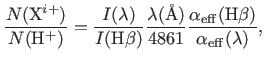
Using the effective recombination coefficients, we determine ionic abundances, X${}^{i+}$ /H${}^{+}$ , from the measured intensities of ORLs as follows:

$$\frac{N({\rm X}^{i+})}{N({\rm H}^{+})}=\frac{I({\lambda})}{I({{\r... ...}})}{4861} \frac{\alpha_{\rm eff}({\rm H}\beta)}{\alpha_{\rm eff}(\lambda)}, %$$ (1)

where $I({\lambda})$ is the intrinsic line flux of the emission line $\lambda$ emitted by ion ${\rm X}^{i+}$ , $I({{\rm H}\beta})$ is the intrinsic line flux of H$\beta$ , $\alpha_{\rm eff}({\rm H}\beta)$ the effective recombination coefficient of H$\beta$ , and $\alpha_{\rm eff}(\lambda)$ the effective recombination coefficient for the emission line $\lambda$ .

Abundances of helium and carbon from ORLs are given in Table 6. We derived the ionic and total helium abundances from HeI $\lambda$ 4471, $\lambda$ 5876 and $\lambda$ 6678 lines. We assumed the Case B recombination for the HeI lines (Porter et al., 2013; Porter et al., 2012). We adopted an electron temperature of $T_{\rm e}=5\,000$  K from HeI lines, and an electron density of $N_{\rm e}=1000$  cm${}^{-3}$ . We averaged the He${}^{+}$ /H${}^{+}$ ionic abundances from the HeI $\lambda$ 4471, $\lambda$ 5876 and $\lambda$ 6678 lines with weights of 1:3:1, roughly the intrinsic intensity ratios of these three lines. The total He/H abundance ratio is obtained by simply taking the sum of He${}^{+}$ /H${}^{+}$ and He${}^{2+}$ /H${}^{+}$ . However, He${}^{2+}$ /H${}^{+}$ is equal to zero, since HeII $\lambda$ 4686 is not present. The C$^{2+}$ ionic abundance is obtained from C II $\lambda$ 6462 and $\lambda$ 7236 lines.

Table 6: Empirical ionic abundances derived from ORLs.

Ion	$\lambda$ (Å)	Mult	Value $^{\mathrm{a}}$
He$^+$	4471.50	V14	0.141
	5876.66	V11	0.121
	6678.16	V46	0.115
	Mean		0.124
He$^{2+}$	4685.68	3.4	0.0
He/H			0.124
C$^{2+}$	6461.95	V17.40	3.068($-3$ )
	7236.42	V3	1.254($-3$ )
	Mean		2.161($-3$ )

$^{\mathrm{a}}$

Assuming $T_{\rm e}=5\,000$ K and $N_{\rm e}=1000$ ${\rm cm}^{-3}$ .

4.3 Ionic and total abundances from CELs

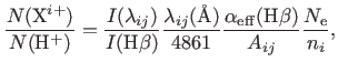
We determined abundances for ionic species of N, O, Ne, S and Ar from CELs. To deduce ionic abundances, we solve the statistical equilibrium equations for each ion using EQUIB code, giving level population and line sensitivities for specified $N_{\rm e}=1000$  cm${}^{-3}$ and $T_{\rm e}=10\,000$  K adopted according to our photoionization modeling. Once the equations for the population numbers are solved, the ionic abundances, X${}^{i+}$ /H${}^{+}$ , can be derived from the observed line intensities of CELs as follows:

$$\frac{N({\rm X}^{i+})}{N({\rm H}^{+})}=\frac{I(\lambda_{ij})}{I({... ...)}{4861} \frac{\alpha_{\rm eff}({{\rm H}\beta})}{A_{ij}} \frac{N_{\rm e}}{n_i},$$ (2)

where $I(\lambda_{ij})$ is the dereddened flux of the emission line $\lambda_{ij}$ emitted by ion ${\rm X}^{i+}$ following the transition from the upper level $i$ to the lower level $j$ , $I({{\rm H}\beta})$ the dereddened flux of H$\beta$ , $\alpha_{\rm eff}({{\rm H}\beta})$ the effective recombination coefficient of H$\beta$ , $A_{ij}$ the Einstein spontaneous transition probability of the transition, $n_i$ the fractional population of the upper level $i$ , and $N_{\rm e}$ is the electron density.

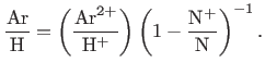
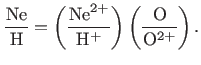
Total elemental and ionic abundances of nitrogen, oxygen, neon, sulfur and argon from CELs are presented in Table 7. Total elemental abundances are derived from ionic abundances using the ionization correction factors ($icf$ ) formulas given by Kingsburgh & Barlow (1994). The total O/H abundance ratio is obtained by simply taking the sum of the O$^{+}$ /H$^{+}$ derived from [O II] $\lambda\lambda$ 3726,3729 doublet, and the O$^{2+}$ /H$^{+}$ derived from [O III] $\lambda\lambda$ 4959,5007 doublet, since HeII $\lambda$ 4686 is not present, so O${}^{3+}$ /H${}^{+}$ is negligible. 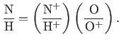The total N/H abundance ratio was calculated from the N$^{+}$ /H$^{+}$ ratio derived from the [N II] $\lambda\lambda$ 6548,6584 doublet, correcting for the unseen N$^{2+}$ /H$^{+}$ using,

$$\footnotesize \frac{{\rm N}}{{\rm H}}=\left(\frac{{\rm N}^{+}}{{\rm H}^{+}}\right) \left(\frac{{\rm O}}{{\rm O}^{+}}\right).$$ (3)

The Ne$^{2+}$ /H$^{+}$ is derived from [Ne III] $\lambda$ 3869 line. Similarly, the unseen Ne$^{+}$ /H$^{+}$ is corrected for, using

$$\frac{{\rm Ne}}{{\rm H}}=\left(\frac{{\rm Ne}^{2+}}{{\rm H}^{+}} \right) \left(\frac{{\rm O}}{{\rm O}^{2+}}\right) .$$ (4)

For sulfur, we have S$^{+}$ /H$^{+}$ from the [S II] $\lambda\lambda$ 6716,6731 doublet and S$^{2+}$ /H$^{+}$ from the [S III] $\lambda$ 9069 line. The total sulfur abundance is corrected for the unseen stages of ionization using

$$\footnotesize \frac{{\rm S}}{{\rm H}}=\left(\frac{{\rm S}^{+}}{{\... ...} \right) \left[1-\left(1-\frac{{\rm O}^{+}}{{\rm O}}\right)^{3}\right]^{-1/3}.$$ (5)

The [Ar III] 7136 line is only detected, so we have only Ar$^{2+}$ /H$^{+}$ . The total argon abundance is obtained by assuming Ar$^{+}$ /Ar = N$^{+}$ /N:

$$\footnotesize \frac{{\rm Ar}}{{\rm H}}=\left(\frac{{\rm Ar}^{2+}}{{\rm H}^{+}} \right) \left(1-\frac{{\rm N}^{+}}{{\rm N}}\right)^{-1}.$$ (6)

As it does not include the unseen Ar$^{3+}$ , so the derived elemental argon may be underestimated.

Figure: Ionic abundance maps of Abell 48. From left to right: spatial distribution maps of singly ionized Helium abundance ratio He${}^{+}$ /H${}^{+}$ from HeI ORLs (4472, 5877, 6678); ionic nitrogen abundance ratio N${}^{+}$ /H${}^{+}$ ( $\times 10^{-5}$ ) from $[$ N II$]$ CELs (5755, 6548, 6584); ionic oxygen abundance ratio O${}^{2+}$ /H${}^{+}$ ( $\times 10^{-4}$ ) from $[$ O III$]$ CELs (4959, 5007); and ionic sulfur abundance ratio S${}^{+}$ /H${}^{+}$ ( $\times 10^{-7}$ ) from $[$ S II$]$ CELs (6716, 6731). North is up and east is toward the left-hand side. The white contour lines show the distribution of the narrow-band emission of H$\alpha$ in arbitrary unit obtained from the SHS.
(A color version of this figure is available in the online journal.)

Fig.4 shows the spatial distribution of ionic abundance ratio He${}^{+}$ /H${}^{+}$ , N${}^{+}$ /H${}^{+}$ , O${}^{2+}$ /H${}^{+}$ and S${}^{+}$ /H${}^{+}$ derived for given $T_{\rm e}=10000$ K and $N_{\rm e}=1000$ cm$^{-3}$ . We notice that both O${}^{2+}$ /H${}^{+}$ and He${}^{+}$ /H${}^{+}$ are very high over the shell, whereas N${}^{+}$ /H${}^{+}$ and S${}^{+}$ /H${}^{+}$ are seen at the edges of the shell. It shows obvious results of the ionization sequence from the highly inner ionized zones to the outer low ionized regions.

Table 7: Empirical ionic abundances derived from CELs.

Ion	$\lambda$ (Å)	Mult	Value $^{\mathrm{a}}$
N${}^{+}$	6548.10	F1	1.356($-5$ )
	6583.50	F1	1.486($-5$ )
	Mean		1.421($-5$ )
	$icf$ (N)		3.026
N/H			4.299($-5$ )
O${}^{+}$	3727.43	F1	5.251($-5$ )
O${}^{2+}$	4958.91	F1	1.024($-4$ )
	5006.84	F1	1.104($-4$ )
	Average		1.064($-4$ )
	$icf$ (O)		1.0
O/H			1.589($-4$ )
Ne${}^{2+}$	3868.75	F1	4.256($-5$ )
	$icf$ (Ne)		1.494
Ne/H			6.358($-5$ )
S${}^{+}$	6716.44	F2	4.058($-7$ )
	6730.82	F2	3.896($-7$ )
	Average		3.977($-7$ )
S${}^{2+}$	9068.60	F1	5.579($-6$ )
	$icf$ (S)		1.126
S/H			6.732($-6$ )
Ar${}^{2+}$	7135.80	F1	9.874($-7$ )
	$icf$ (Ar)		1.494
Ar/H			1.475($-6$ )

$^{\mathrm{a}}$

Assuming $T_{\rm e}=10\,000$ K and $N_{\rm e}=1000$ ${\rm cm}^{-3}$ .